Full Text Search in SmithDB: Designing an Inverted Index for Object Storage
LangChain
Jun 10, 2026
Originally published on langchain.com
Overview
SmithDB supports full-text search and JSON filtering over agent traces with a median (P50) latency of 400 ms, even though the underlying data consists of large, deeply nested JSON documents stored in object storage.
Full-text search is well-trodden ground. Lucene is two decades old; Tantivy and Quickwit have already pushed search and indexing onto object storage. However, when building text search into SmithDB, we decided to approach the problem from first principles because indexing agent traces for search workloads presents a unique challenge.
SmithDB requires a different approach to search
Challenge 1: Unique data characteristics of agent traces
Every LangSmith event encodes the fields inputs and outputs as the overwhelming majority of its total bytes. 1 MB+ payload sizes for inputs and outputs are common, with some of these stretching to hundreds of megabytes uncompressed. These content columns dwarf the identity, timestamp, and other metadata columns by orders of magnitude.
Additionally, as mentioned in the original SmithDB blogpost, the payloads associated with agent traces continue to increase in size over time. This is direct result of LLM context window sizes growing larger and agents running for longer time horizons, causing LLMs to accumulate more context.
These characteristics invert the usual economics of a search index. A traditional log engine indexes billions of small documents, so the index is small relative to each document. We index billions of enormous documents, where one document can produce more index data than many small log lines. Typically the source:index ratio for logs is about to 1:1.25. However for agent traces in LangSmith, we observed the average to be closer to 1:1.9. Three things follow:
- A content filter without an index is catastrophically slow. "Find runs whose tool output mentions a timeout" cannot scan every payload in the candidate range otherwise it would scan many gigabytes to return three rows.
- Term frequencies follow a Zipfian distribution. Natural-language and JSON payloads follow a power law: a handful of tokens (
"agents","import", "role", "type", ubiquitous keys) appear in nearly every document, while the long tail of terms appear once or twice. The index must stay compact and prunable across many orders of magnitude of term frequency, all inside one file. - Multiple query modalities matter. Users query by path ("does this run have
inputs.content.messages?"), by value ("…where it mentionsAlex"), and by free text ("…mentions a latency regression anywhere").
An inverted index is what prevents a content query from performing a full payload scan, and it has to absorb heavy, skewed, semi-structured payloads.
Challenge 2: Object storage
SmithDB keeps all durable data in object storage so compute is relatively stateless and the system scales by adding nodes without having to manage local disks.
The cost of a query is roughly proportional to (requests issued to object storage) × (bytes read per request). On object storage:
- Each object store request carries tens of milliseconds to hundreds of milliseconds of latency.
- Per-request throughput is modest, so fetching a large postings list or positions list before you know you need it can dominate the query.
Every aspect of SmithDB’s inverted index, from its storage layout to query execution is designed with these constraints in mind.
SmithDB search query shapes
Before going deeper into the storage layout for our inverted index, let’s go over the main query patterns the index has to answer. SmithDB's query surface boils down to three predicate families, and they differ in what they match against and what pattern syntax they admit.
- The first is path existence (
json_key): does this document contain key K? For examplejson_key(inputs, "author.name")asks which documents mentionauthor.name. Path existence also supportsLIKEon the key path itself:json_key(inputs, "author.%")orjson_key(inputs, "%.user_id")is a first-class query. Patterns can land anywhere in the path (prefix, suffix, infix). - The second is keyed value (
json_key_search): does key K have a value matching V?json_key_search(inputs, "author.name", "Jane")is the canonical form. The query may be a single token or a multi-token phrase (json_key_search(inputs, "title", "latency regression")), and the phrase variant adds adjacency:"latency regression"matches only documents where those words appear consecutively, not anywhere in the value. - The third is full-text search (
search): does any indexed value match Q?search(error, "timeout")searches a text column directly;search(inputs, "latency regression")searches across every JSON value, regardless of path.
To summarize:
| Shape | What it matches |
|---|---|
| json\_key | key path exists |
| json\key\search | path + value |
| search | text column or any JSON value |
Every later section refers back to this table: when we say "path-only query" we mean json\key, "keyed value" means` jsonkey_search, and "full-text" means search`.
An overview of inverted indexes
An inverted index is the data structure powering every search library, from Lucene to Tantivy. It is like the index at the back of a textbook: look up a term once and jump straight to the pages that mention it instead of reading every page. SmithDB builds on this idea and specializes the storage layout for the large agent-trace payloads it stores in object storage.
Terms, postings, positions
The inverted index structure rests on three concepts:
- a term is the unit we index: a JSON path, a keyed value, or a text token
- a posting is the sorted set of document IDs that contain a term
- a position is where in a document a term appears, which is what makes phrase search possible.
Take five traces indexed on their text:
doc 0: "langchain agents emit traces"
doc 1: "langsmith engine runs deep agents"
doc 2: "langchain deep agents workflow"
doc 3: "agents emit deep langsmith traces"
doc 4: "deep langsmith powers the engine"
The index keeps one entry per term, pointing at the documents that mention it:
term         posting list      positions
──────────   ──────────────    ─────────────────────────
agents       [0, 1, 2, 3]      0:[1]  1:[4]  2:[2]  3:[0]
deep         [1, 2, 3, 4]      1:[3]  2:[1]  3:[2]  4:[0]
emit         [0, 3]            0:[2]  3:[1]
engine       [1, 4]            1:[1]  4:[4]
langchain    [0, 2]            0:[0]  2:[0]
langsmith    [1, 3, 4]         1:[0]  3:[3]  4:[1]
powers       [4]               4:[2]
runs         [1]               1:[2]
the          [4]               4:[3]
traces       [0, 3]            0:[3]  3:[4]
workflow     [2]               2:[3]
Each term is one dictionary entry: look up the value, read its posting list, and you know exactly which documents to fetch. A query like search("deep agents") intersects the posting lists for deep ([1, 2, 3, 4]) and agents ([0, 1, 2, 3]) to get [1, 2, 3] with no payload scan.
The positions column records, per document, the token offset(s) where the term appears, e.g. 1:[0] means doc 1, position 0. That is what makes phrase search possible: search("langsmith engine") matches doc 1 because langsmith is at offset 0 and engine at offset 1 (0 + 1 == 1), but not doc 4, where powers and the sit between them (langsmith at 1, engine at 4).
Why we leveraged Vortex and not Tantivy
Tantivy is an excellent search indexing library and the obvious reference point for Lucene-style search in Rust. We started by asking whether we could adopt it directly. The design we ended up with is heavily inspired by Tantivy, but a few constraints made it an awkward fit for our use-case directly:
1. Object storage, not local disk. Tantivy is built around mmap; every byte is microseconds away and random I/O is effectively free. We're on object storage with ~100 ms round trips, where layout and coalescing decide query latency, not CPU.
2. Embedded in a columnar engine. SmithDB queries run through Apache DataFusion over Vortex. We wanted search to push down through the same scan pipeline as every other predicate, not run as a parallel query stack with its own segment model and IO assumptions.
3. Doc IDs aligned with Vortex rows. Tantivy's writer assigns its own segment-local doc IDs in insertion order and renumbers them on every merge. SmithDB needs the index to point directly at row positions in the corresponding Vortex data file (we use Vortex for our core event data files), so a doc ID is a row index — no translation table, no second identity to reconcile at query time, and merges that follow the data file's row ordering need no remap. Additionally, our compaction remaps the row positions which also doesn’t work well with Tantivy’s index merge as we’ll detail in the second part of this blog post.
Our journey to develop SmithDB’s inverted index
Quick primer on Vortex
Vortex is an extensible and columnar file format SmithDB uses for object storage. Unlike fixed formats such as Parquet, Vortex allows pluggable encodings and custom file layouts which lets us tailor compression and I/O access patterns to our workload without forking the file format.
Every read prunes entire row groups using statistics, filters surviving rows down to a mask, and projects only the columns the query actually needs.
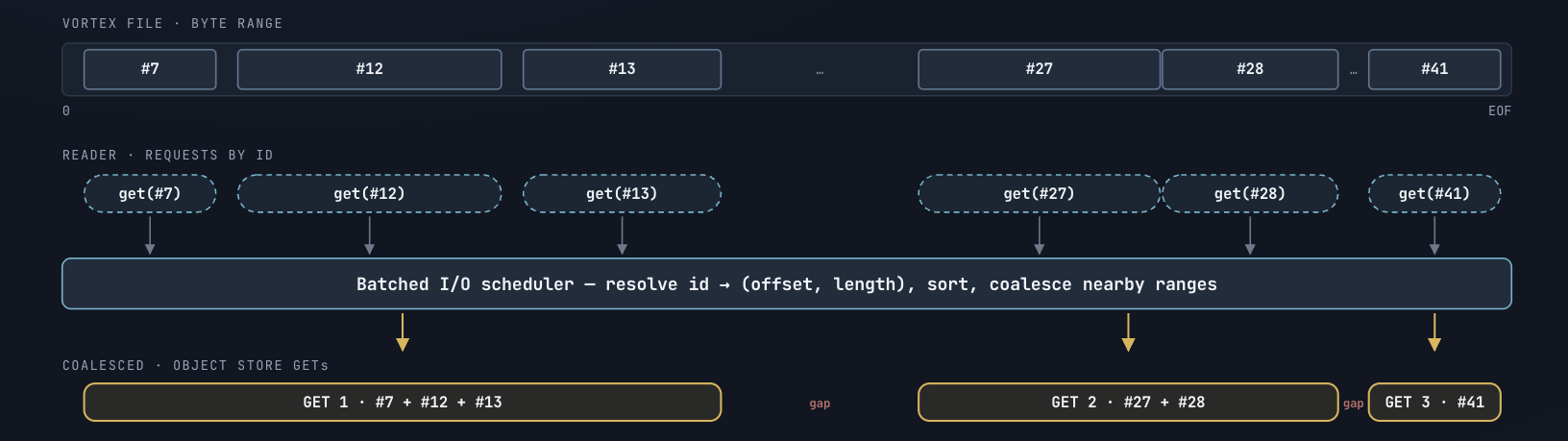
The unit of I/O in a Vortex file is a segment: a contiguous physical byte range. On object storage a round-trip costs roughly 100 ms, so the primary lever for query latency is minimizing the number of requests. Vortex's I/O scheduler coalesces nearby segment reads into a single request, merging reads within a 1 MB gap into one, up to a 16 MB window, so sequential access patterns in the index map to very few object store GETs.
Our (unsuccessful) first attempt
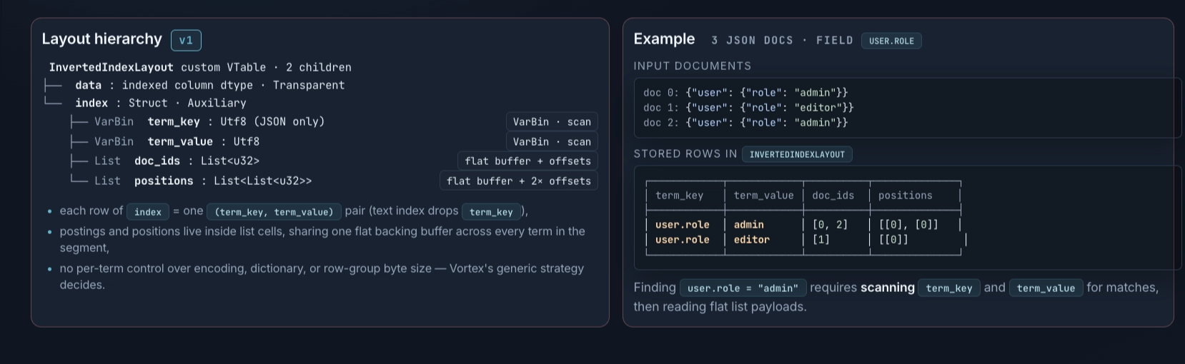
The first version was a near-literal translation of the textbook inverted index. Two columns (term_key for paths and term_value for tokens) lets one layout serve all three query shapes: path-existence read term_key, keyed search intersected postings across both columns, and full-text intersected on term_value alone. Postings were stored as List<u32> cells, positions as List<List<u32>>.
We leaned on Vortex's defaults: FSST encoding for the term columns, bitpacked encoding for postings and positions, and a zoned storage layout that allowed for pruning at query time. Positions (required for phrase search) alone were an order of magnitude larger than every other column, so we kept the index in a separate file from the core run data. This let us decouple index construction and merge from the core write path. Vortex's APIs work on row indices and masks, so delegating index filtering to a sibling file composed naturally.
Three problems showed up at scale:
- No per-term encoding control. Vortex picked the encoding for the whole column, not per term, so a single common token (
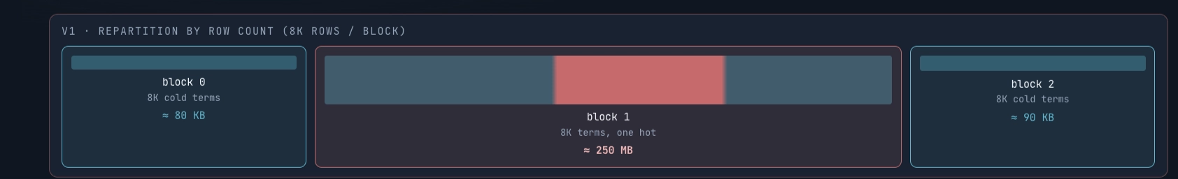
agent,langchain) forces a larger bit width on every term in the entire chunk, leading to poor bitpacking. The rest of the column paid for it with worse cache behavior and larger reads, and we had no lever to apply more aggressive bitpacking selectively to high-frequency terms. - Fixed-size row groups were blind to term skew. We batched a fixed number of terms per row group, which meant a single high-frequency term could push one row group past 100 MB compressed while another sat at a few MB. At query time that turned into one outsized object-store GET; at merge time it turned into outsized in-memory decode.
- Merge had to reshape positions. Merging two segments meant decoding the full positions
List<List<u32>>, reshuffling inner lists into the new document order, and recomputing every outer offset. CPU time and allocations both spiked on compaction. For an index where 70%+ of bytes are positions, this was the dominant compaction cost.
Second attempt: V2 Inverted index storage layout
Our v2 layout addresses all three v1 problems by changing the unit of organization from "N terms per row group" to a byte-budgeted row group, and by owning the byte layout per column instead of directly relying on Vortex defaults. The rest of this section walks through the new unit of organization, what lives inside it, and the encoding choices that earned the byte budget.
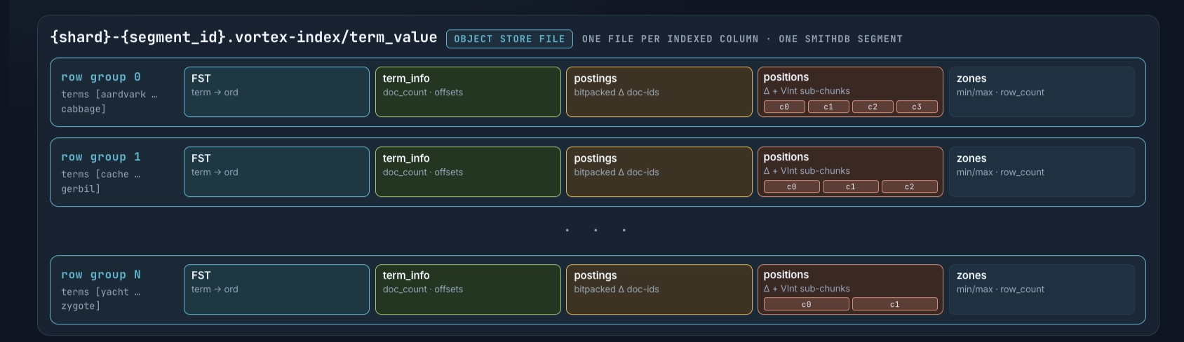
Row groups, sized in bytes
Since a row group is the unit of pruning and I/O, we determine the row group sizes with fixed independent byte budgets instead of a fixed row count.
- 32 MB of posting bytes: bounds the worst-case object-store GET when a query reads postings for a row group.
- 64 MB of raw term-string bytes: caps raw bytes per row group.
Sizing in bytes, not term count, is what fixes v1's third problem. Term skew makes term count a poor proxy for IO size, as one high-frequency term in a v1 row group could push it past even 500 MB compressed. The byte budgets give us an upper bound on every row group for the amount of bytes fetched from object store or memory footprint while executing queries.
Per-row-group min/max/count via a zoned storage layout on the term column lets the query planner skip entire row groups before touching the FST. For path queries that target a specific prefix this is the single biggest saving: most row groups simply don't contain anything in the predicate's range.
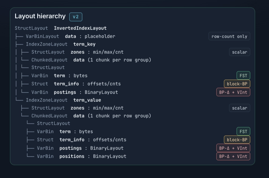
Inside one row group
Each row group carries four columns (three for term_key, which skips positions):
term— a binary layout whose bytes are an FST ( **finite state transducer** ) mapping each term to an ordinal (its row index inside this row group). Our usage of FSTs is inspired by Tantivy.term_info— term metadata: doc count plus offsets intopostingsandpositions.postings— binary blob. Per-term lists are split into 128-doc blocks of bitpacked deltas with aVInttail for the leftover < 128 docs.positions— binary blob, same encoding. Only present onterm_value; path existence is a document-level question, soterm_keyskips this column entirely.
A lookup is one walk through the dictionary, one offset table read, and one byte-range fetch. The FST resolves the term to an ordinal. The ordinal indexes into term_info, which gives an offset into postings and (for phrase queries) an offset into positions. The query reads those byte ranges directly. No payload scan, no nested-list decode, and because each column is its own chunked layout, a non-phrase query fetches just term \+ term_info \+ postings and never opens the positions column.
Encoding choices
We use FST for the term dictionary. We compared FST against the obvious alternatives (Vortex's default FSST string encoding, prefix-shared keep_add, and plain zstd) on a representative row group with 2.79M term occurrences. The shape of the win depends on cardinality:
| Column | Unique terms | Raw | FSST | zstd | FST |
|---|---|---|---|---|---|
| term\_key (JSON paths) | 546 | 88.8 MiB | 34.7 MiB | 16.3 KiB | 3.8 KiB |
| term\_value (token values) | 1.41M | 55.1 MiB | 65.7 MiB | 21.7 MiB | 32.7 MiB |
| term\value:term\key combined | 2.79M | 146.6 MiB | 81.7 MiB | 31.3 MiB | 37.6 MiB |
On term_key, where a few hundred JSON paths repeat across millions of rows, the FST collapses the entire dictionary to 3.8 KiB: four orders of magnitude smaller than the raw bytes and ~4× smaller than zstd. On the high-cardinality term_value column, FST is ~1.5× larger than zstd but still beats FSST. The crucial point is that zstd is opaque: every lookup requires decompressing the block. The FST is the index itself — exact lookup, prefix and range scans, and automaton walks (LIKE, fuzzy, regex) all run directly against the compressed bytes with O(|term|) cost and no hashing.
We also fold the keyed-search and full-text query shapes into a single FST per row group by storing term_value entries as {token}\0{flattened_path}. Keyed search becomes exact FST lookup; full-text search becomes a prefix scan on token\0, walking every path the token appears under.
We use block-bitpacked deltas per term. Postings and positions both use the same Tantivy/Lucene-style two-tier encoding. The shape of the encoding is what makes per-term control possible and what makes merge cheap.
Each per-term list is split into fixed 128-element blocks plus a tail of < 128 leftovers:
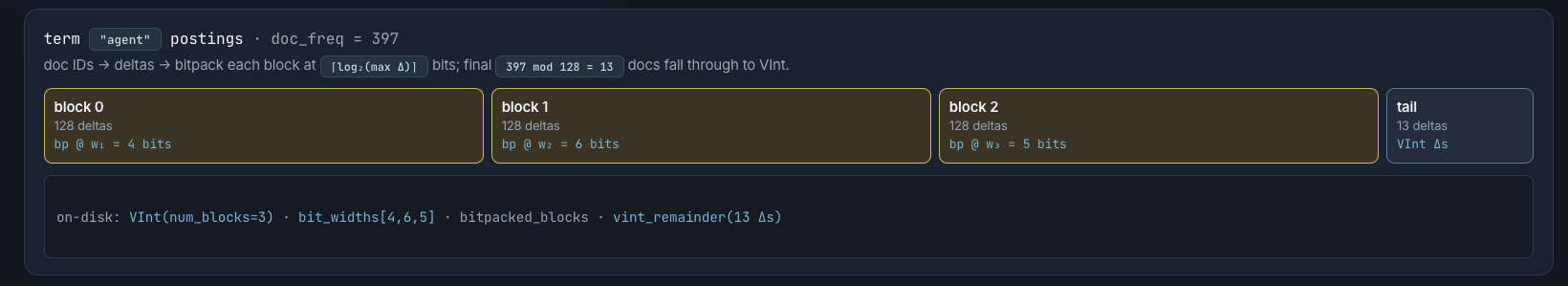
Within a block we store deltas between successive doc IDs, not the IDs themselves, and bitpack the block to the minimum width that fits its max delta. A dense, regular run of IDs packs down to just a few bits each. The trailing partial block (by definition rare for high-frequency terms, and the entire posting list for low-frequency ones) falls back to VInt, ~1 byte per small delta, degrading gracefully on the long tail.
Two properties fall out of it that the v1 List<u32> encoding didn't have:
1. Per-term encoding, not per-column. Each term picks its own bit widths block-by-block: a frequent term like agent packs at 3–4 bits per doc, a rare term never leaves its VInt tail. v1 forced one width across the whole column, so frequent terms inflated everyone's bytes.
2. Opaque to Vortex. Vortex sees the encoded bytes as a single binary blob; it never decodes them into Arrow on the read path. That's what lets a query fetch just the byte range it needs, decode blocks on demand, and skip-decode past everything the skip list rules out.
Where we diverge from Tantivy with FST usage
Tantivy also leverages FSTs, but builds one FST per segment with sharded partitioning. We build one FST per row group. A row-group-sized FST is small enough that the writer streams through it without ever holding a segment-wide FST in memory, and zone-level pruning skips most row groups before any FST work happens at query time. The trade-off is that a single lookup may touch multiple FSTs per file, but pruning makes that cost rare in practice; the surviving FSTs are small enough that the walks are cheap.
What’s next
In part 2, we’ll explore how we implemented inverted index construction and merging, as well as how we leverage the index in our read path.
//
We’re building SmithDB to solve the systems problems that come with agent observability. If that kind of infrastructure work sounds interesting, _we’re hiring_ .
Read the full article on langchain.com
Published by LangChain on Jun 10, 2026.
OpenCraft Services
Need AI systems like these for your business?